Notes/Introduction to Machine Learning/Introductory lecture.md

type
theoretical

We're gonna be doing

• General intro
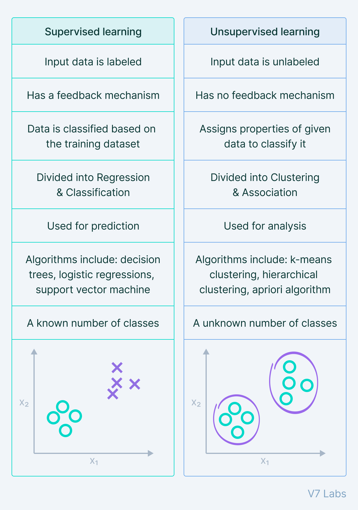
• Unsupervised learning
• Supervised learning

Philosophical Introduction

• What is intelligence?
• Can machines ever be intelligent?

Intelligent systems

a system that can:

• Perceive Interaction with the environment. e.g. computer vision, speech recognition

• Make decisions process incoming information, analyze it, and make decisions based on it. e.g. self-driving cars, game playing

• Learn improve performance over time, i.e. data driven adaptation based on observations only (for unsupervised learning) or based on observations and feedback (for supervised learning)

Relevant Mathematical Notation

Models are noted as m = \gamma (D), where D is the data and \gamma is the model.

Example - a model that predicts the price of a house based on its size and location:

m = \gamma ( \beta_0 + \beta_1 x_1 + \beta_2 x_2)

where x_1 is the size of the house and x_2 is the location of the house.

Unsupervised learning

• Compression Represent all the data in a more compact form (few features)

• Clustering Identify groups of similar data points

• Reduction Reduce the dimensionality of the data, i.e. represent large amount of data by few prototypes¹

The above aims define a cost function or optimization strategy, which is used to teach the machine to learn, but thee is no feedback from the environment. (hence unsupervised learning).

Example:

Consider a dataset of images of cats and dogs. We can use unsupervised learning to identify the features that are common to all cats and all dogs. This can be used to classify new images of cats and dogs.

Supervised learning

Classification/Regression

Data: observations, e.g. images, text, etc. and labels, e.g. cat/dog, spam/not spam, etc.

Regression problems:

• Predict quantitative values, e.g. house prices, stock prices, etc.

e.g. predict the weight of a cow based on its size:

m = \gamma ( \beta_0 + \beta_1 x_1)

where x_1 is the size of the cow.

Classification problems:

• Predict qualitative values, e.g. cat/dog, spam/not spam, etc.
• Binary classification: two classes
• Multi-class classification: more than two classes

Important

It is crucial to find the right features to represent the data. The model is only as good as the features used to represent the data.

Some issues

• Complexity of the model
• Parametrization² of a hypothesis
• Noise in the dataset

Other forms of learning

• Semi-supervised learning, self-supervised learning

Partially labeled data, e.g. some images are labeled, some are not. Extend by making predictions on the unlabeled data and using the predictions to improve the model.

• Reinforcement learning Delayed reward (feedback) from the environment. e.g. game playing, robotics, etc.

• Transfer learning, few-shot learning, single-shot learning

Use knowledge from one task to improve performance on another task. e.g. use knowledge from a large dataset to improve performance on a smaller dataset.

Deeper look of reinforcement learning

There's a reward signal evaluating the outcome of past actions.

Problems involving an agent³, an environment, and a reward signal.

The goal is to learn a policy that maximizes the reward signal.

graph TD
    A[Agent] --> B[Environment]
    B --> C[Reward signal]
    C --> A

Mathematical Formulation

Markov Decision Process⁴ (MDP) is a mathematical framework for modeling decision-making in situations where outcomes are partly random and partly under the control of a decision maker.

An MDP consists of:

• A set of states S
• A set of actions A
• A reward function R
• A transition function P
• A discount factor \gamma

It can be represented as a tuple (S, A, R, P, \gamma). Or a graph:

graph TD
    A[States] --> B[Actions]
    B --> C[Reward function]
    C --> D[Transition function]
    D --> E[Discount factor]

The process itself can be represented as a sequence of states, actions, and rewards:

(s_0, a_0, r_0, s_1, a_1, r_1, s_2, a_2, r_2, \ldots)

The goal is to learn a policy \pi that maps states to actions, i.e. \pi(s) = a.

The policy can be deterministic or stochastic⁵.

1. At time step t=0, the agent observes the current state s_0.
2. For t=0 until end:
   • The agent selects an action a_t based on the policy \pi.
   • Environment grants reward r_t and transitions to the next state s_{t+1}.
   • Agent updates its policy based on the reward and the next state.

To summarize:

G_t = \Sigma_{t\geq 0}y^t r_t = r_t + \gamma r_{t+1} + \gamma^2 r_{t+2} + \ldots

where G_t is the return at time step t, r_t is the reward at time step t, and \gamma is the discount factor.

The value function

The value function V(s) is the expected return starting from state s and following policy \pi.

V_\pi(s) = \mathbb{E}_\pi(G_t | s_t = s)

Similarly, the action-value function Q(s, a) is the expected return starting from state s, taking action a, and following policy \pi.

Q_\pi(s, a) = \mathbb{E}_\pi(G_t | s_t = s, a_t = a)

Bellman equation

Like Richard Bellman from the Graph Algorithms.

States that the value of a state is the reward for that state plus the value of the next state.

V_\pi(s) = \mathbb{E}_\pi(r_{t+1} + \gamma V_\pi(s_{t+1}) | s_t = s)

Q-learning

Something makes me feel like this will be in the exam.

The goal of Q-learning is to find the optimal policy by learning the optimal Q-values for each state-action pair.

What's a Q-value? It's the expected return starting from state s, taking action a, and following policy \pi.

Q^*(s, a) = \max_\pi Q_\pi(s, a)

The optimal Q-value Q^*(s, a) is the maximum Q-value for state s and action a. The algorithm iteratively updates the Q-values based on the Bellman equation. This is called value iteration.

Conclusion

As with every other fucking course that deals with graphs in any way shape or form, we have to deal with A FUCK TON of hard-to-read notation <3.

---

1. Prototypes in this context means a representative sample of the data. For example, if we have a dataset of images of cats and dogs, we can represent the dataset by a few images of cats and dogs that are representative of the whole dataset. ↩︎

2. Parametrization is the process of defining a model in terms of its parameters. For example, in the model m = \gamma ( \beta_0 + \beta_1 x_1), \beta_0 and \beta_1 are the parameters of the model. ↩︎

3. An agent is an entity that interacts with the environment. For example, a self-driving car is an agent that interacts with the environment (the road, other cars, etc.) to achieve a goal (e.g. reach a destination). ↩︎

4. https://en.wikipedia.org/wiki/Markov_chain ↩︎

5. A deterministic policy maps each state to a single action, while a stochastic policy maps each state to a probability distribution over actions. For example, a deterministic policy might map state s to action a, while a stochastic policy might map state s to a probability distribution over actions. ↩︎